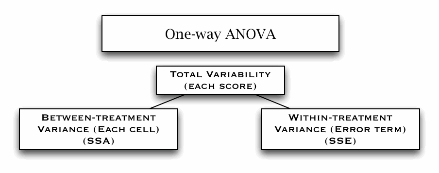
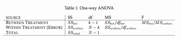
Basics
Basic math calculations (W1)
Measures for central tendency (W1)
One-sample t-test (W2)
Correlation and Regression (W3)
Comparing two means (t-test) (W4)
More correlation (W5)
Multiple regressions (W6)
Effect size (W7)
One-way ANOVA (W8)
Planned comparisons and post-hoc test (W9)
Two-way Factorial ANOVA (W10)
Two-way Repeated Measure ANOVA (W11)
Mixed-design ANOVA (W12)
Non-parametric tests (W13)
Three-way ANOVA
Multilevel Liniear (mixed-effects) Model
Data management
Graphics
Distributions
Time Series
Using R for statistical analysis

Last update:
- This document was compiled from various sources by Tomonori Nagano (tnagano@lagcc.cuny.edu). Please let me know if you find any error.
- See here for the RMarkdown output.
- Download the data files here.
Basics
Clear cache
# clear the cache
rm(list = ls())
Installing packages
# the repositiory PA1 seems to be most stable (http://lib.stat.cmu.edu/R/CRAN)
install.packages(c("psych","gdata","reshape","xtable","gplots","nlme","foreign","ez"))
Check R/package versions
getRversion()
package-version("psych")
Saving history
# save hisotry
savehistory("name.Rhistory")
loadhistory("name.Rhistory")
Loading packages or data
# loading a package or data set
library()
data()
Show the data structure
str(dataFrameName)
Formatting text output
string <- "This is a sample string"
cat(substring(string,1,10),substring(string,15,19),"\n",sep="\t")
cat("Roots of two: ",format(2^(1:10),digit=2),"\n")
Array and matrices
# make a matrix with array or matrix
matrix1 <- array(1:10, dim=c(2,5))
matrix2 <- matrix(1:10,2,5)
matrix3 <- 1:10; dim(array3) <- c(2,5)
class(matrix1)

# numbers are recycled if the number of cells is larger
array(1:10, dim=c(5,10))
Matrix calculus
# this performs cell-by-cell calculation
m1 <- array(1:10, dim=c(2,5))
m1 + m1
m1 * m1

# matrix calculus from J.Penzer's note (2006)
m4 <- array(1:3, c(4,2))
m5 <- array(3:8, c(2,3))
m4 %*% m5
m6 <- array(c(1,3,2,1),c(2,2))
m6
v1 <- array(c(1,0), c(2,1))
solve(m6,v1)
solve(m6) # inverts m6
# does the same as solve(m6,v1)
solve(m6) %*% v1
Using functions
# functionName <- function(arg1,arg2=DEFAULT,...) {expression}
# see the basic calculations for examples
Change the default options (print width, number/format of digits)
# change the default width
width.default <- getOption("width"); options(width=120)

# restoring default
options(width=width.default)

# changing the number of digits
options(digits=7)

# put biase toward non-scientific notations
options(scipen=3)
Running r scripts from command-line
# ~/home$ R CMD BATCH r.script (>output.file)
$ cd Documents/rDocument/
$ R CMD BATCH Rprocedure.r
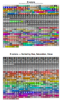
R colors
# list of all color names
# also see ?palette
colors()

# different color combo
colors3 <- c("lightblue","lightyellow","lightgreen")
colors5 = c("#A6CEE3","#1F78B4","#B2DF8A","#33A02C","#FB9A99")

# pre-set color functions
# it looks better to set the alpha level to less than 1
rainbow(10)
heat.colors(10, alpha = 1)
terrain.colors(10, alpha = 1)
topo.colors(10, alpha = 1)
cm.colors(10, alpha = 1)

# with color brewer
library(RColorBrewer)
display.brewer.all() # show all pre-set colors
colorRampPalette(brewer.pal(9,"Blues"))(15) # for more than 9 colors
display.brewer.pal(6,"BuGn")
brewer.pal(6,"BuGn")
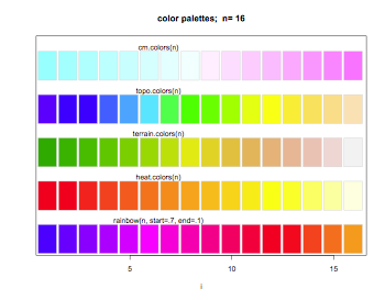
R colors (from help file)
##------ Some palettes ------------
demo.pal <- function(n, border = if (n<32) "light gray" else NA,
         main = paste("color palettes;  n=",n),
         ch.col = c("rainbow(n, start=.7, end=.1)", "heat.colors(n)",
         "terrain.colors(n)", "topo.colors(n)","cm.colors(n)")) {
  nt <- length(ch.col)
  i <- 1:n; j <- n / nt; d <- j/6; dy <- 2*d
  plot(i,i+d, type="n", yaxt="n", ylab="", main=main)
  for (k in 1:nt) {
      rect(i-.5, (k-1)*j+ dy, i+.4, k*j,
      col = eval(parse(text=ch.col[k])), border = border)
      text(2*j,  k * j +dy/4, ch.col[k])
  }
}
n <- if(.Device == "postscript") 64 else 16
# Since for screen, larger n may give color allocation problem
demo.pal(n)
Making dummy data
# make a dummy data set
x = c(rep(1,5),rep(2,3),rep(3,5))
y = c(7,5,6,8,4,5,4,6,3,5,4,6,2)
z = rnorm(13,mean=10,sd=5)
thisData = cbind(x,y,z)
thisData = as.data.frame(thisData)
thisData$x = factor(thisData$x)
levels(thisData$x) = c("A","B","C")

summary(thisData)

library(psych)
describe(thisData)

head(thisData)
thisData[1:3,]
Making dummy data (with matrix())
matrix(letters[1:10],nrow=5,ncol=2)
matrix(letters[1:10],nrow=5,ncol=2,byrow=TRUE)
Making dummy data (reconstructing data from SD and mean)
# mean, SD, and n from the published research
mean = 5; SD = 0.8; n = 300
X0 <- rnorm(n)
SE = SD/sqrt(n)
thisData <- cbind(mean+SE*sqrt(length(X0))*(X0-mean(X0)/sd(X0)),"some_level")
mean = 7; SD = 0.5; n = 100
X0 <- rnorm(n)
SE = SD/sqrt(n)
thisData <- rbind(thisData,cbind(mean+SE*sqrt(length(X0))*(X0-mean(X0)/sd(X0)),"another_level"))
thisData <- data.frame(as.numeric(thisData[,1]),thisData[,-1])
colnames(thisData) <- c("value","factor")
head(thisData)
# checking the accuracy
mean(thisData$value)
tapply(thisData$value,thisData$factor,mean)
sd(thisData$value)
tapply(thisData$value,thisData$factor,sd)
For loop (looping different levels)
x = c(rep(1,5),rep(2,3),rep(3,5))
y = c(7,5,6,8,4,5,4,6,3,5,4,6,2)
z = rnorm(13,mean=10,sd=5)
thisData = cbind(x,y,z)
thisData = as.data.frame(thisData)
thisData$x = factor(thisData$x)
levels(thisData$x) = c("A","B","C")

for (i in 1:length(levels(thisData$x))) {
 	print(levels(thisData$x)[i])
  	tempData <- drop.levels(thisData[thisData$x == levels(thisData$x)[i],],reorder=FALSE)
 	print(summary(tempData))
}
For loop (saving the output table into an Excel file)
x = c(rep(1,5),rep(2,3),rep(3,5))
y = c(7,5,6,8,4,5,4,6,3,5,4,6,2)
z = rnorm(13,mean=10,sd=5)
thisData = cbind(x,y,z)
thisData = as.data.frame(thisData)
thisData$x = factor(thisData$x)
levels(thisData$x) = c("A","B","C")

# using the openxlsx package. The xlsx package requires Java and may need an additional step to use.
library(openxlsx)

wb <- createWorkbook("My name here")
for (i in 1:length(levels(thisData$x))) {
	addWorksheet(wb, strtrim(as.character(levels(thisData$x)[i]),15), gridLines = FALSE)
  	tempData <- drop.levels(thisData[thisData$x == levels(thisData$x)[i],],reorder=FALSE)
	writeData(wb, tempData, sheet = i)
}
saveWorkbook(wb, "foo.xlsx")
Read data from files
# For Unix
# setwd('/media/MYUSB/PATH/file.txt')
# For Windows
# setwd('F:/PATH/file.txt')

# from a text file
ratings = read.table("text.txt",sep=" ",header=TRUE)
summary(ratings)

# from SPSS file
library(foreign)
# ratings =  read.spss("spssFile.sav", to.data.frame=TRUE)
ratings =  read.spss("spssFile.sav", to.data.frame=TRUE)
Output with sink() (the layout is aligned)
# change STDOUT
sink("sinkExamp.txt")
i = 1:10
outer(i, i, "*")
sink()
unlink("sink-examp.txt")
Output with write.table()
# printing dataframe or table
x = data.frame(a="a", b=pi)
# sep can be changed to "\t" or " "
write.table(x, file = "foo.csv", sep = ",", col.names = NA, qmethod = "double")
Save plots as PDF
pdf("pdfOutput.pdf", width = 8, height = 6, onefile = TRUE, pointsize = 9)
normal <- rnorm(100,10,10)
t <- rt(100,10)*10
f <- rf(100,10,10)*10
plot(rnorm(100,10,10),col="blue",pch=78)
points(t,col="red",pch=84)
points(f,col="green",pch=70)
dev.off()
Data transformation for RM analyses
# from Reshaping Data with the reshape Package by Hadley Wickham
thisData = rbind(c(4,6,2),c(10,9,8),c(5,4,3),c(8,6,7),c(2,2,2))
thisData = cbind(thisData,c(1,1,1,2,2))
thisData = as.data.frame(thisData)
colnames(thisData) = c("early","mid","late","gender")
thisData$gender = factor(thisData$gender)
levels(thisData$gender) = c("male","female")
thisData

# melting dataframe
library(reshape)
# make a new col to keep the subject id
temp = cbind(thisData,as.factor(rownames(thisData)))
colnames(temp) = c(colnames(thisData),"subject")
moltenData = melt(temp,id=c("subject"))
moltenData
# recovering the original data
# Note: cast() has the default names for variables ('value' and 'variable') and
#       there seems to be no way to change them
cast(moltenData, subject ~ variable)
cast(moltenData, ... ~ variable)
cast(moltenData, ... ~ subject)
cast(moltenData, ... ~ variable + subject)
cast(moltenData, subject ~ value)

# cross tabulating dataframe
crossTabulatedData = xtabs(value ~ subject + variable, data = moltenData)
crossTabulatedData
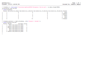
Data transformation (demo of the Field textbook pp.764-767)
library(reshape)

thisData <- read.spss("DiscoveryingStatsSPSS3/Honeymoon Period.sav", to.data.frame=TRUE)
head(thisData)

thisData.molten <- melt(thisData, id=c("Person","Gender"))
head(thisData.molten)
grep
tempIndex = grep("Q[0-9]|midterm|final|pres",colnames(thisData))
newData = drop.levels(thisData[tempIndex,],reorder=FALSE)
summary(newData)
Tables
thisData = read.table("Daphnia.txt",header=TRUE)
attach(thisData)
# means of Growth.rate by Detergent
tapply(Growth.rate,Detergent,mean)

# use list() for two-dimensional tables
# tapply(VALUE,list(ROW,CLUMN),FUNCTION)
tapply(Growth.rate,list(Daphnia,Detergent),mean)

# using an anonymous function
tapply(Growth.rate,list(Daphnia,Detergent), function(x){sqrt(var(x)/length(x))})

# a three-dimensional table
tapply(Growth.rate,list(Daphnia,Detergent,Water),mean)
# and use ftable() to flatten the table
ftable(tapply(Growth.rate,list(Daphnia,Detergent,Water),mean))

# the fourth argument is an option for the function
tapply(Growth.rate,list(Daphnia,Detergent),mean,na.rm=TRUE)

# saving the table data as a dataframe
# (alternatively, use as.data.frame.table())
dets <- as.vector(tapply(as.numeric(Detergent),list(Detergent,Daphnia),mean))
clones <- as.vector(tapply(as.numeric(Daphnia),list(Detergent,Daphnia),mean))
means <- as.vector(tapply(Growth.rate,list(Detergent,Daphnia),mean))
detergent <- levels(Detergent)[dets]
daphnia <- levels(Daphnia)[clones]
data.frame(means,detergent,daphnia)

as.data.frame.table(tapply(Growth.rate,list(Daphnia,Detergent),mean))
Tables (tables of counts)
cells <- rnbinom(10000, size=0.63, prob=0.63/1.83)

# frequency table
table(cells)
gender <- rep(c("male","female"),c(5000,5000))
table(cells,gender)
Converting the frequency table to a dataframe
# see page. 188 of the R book
Probability table
counts <- matrix(c(2,2,4,3,1,4,2,9,1,5,3,3),nrow=4)
prop.table(counts,1)          # index 1 is row-wise
prop.table(counts,2)          # index 2 is column-wise
prop.table(counts)            # no index is table-wise
Permutations and combinations
library(gtools)
# permutation and combination
# n: size of source, r: size of target
# number of permutations: n!/(n-r)!
# number of combinations: n!/(r!*(n-r)!)
x = c("A","B","C","D","E","F")
r = 4
perm = permutations(length(x),r,x,repeats.allowed=FALSE)
perm                         # 360 (6!/(6-4)! = 720/2 = 360)

comb = combinations(length(x),r,x)
comb                         # 15 (6!/4!*(6-4)! = 720/24*2 = 15)
Basic math calculations (W1)
Calculate sum, sumOfSq, sigma, s, and SS
practiceCalculation = function (x) {
    sum = sum(x)                           # sum of vector x
    sumOfSq = sum(x**2)	                   # sum of squares of vector x
    SS = sum((mean(x)-x)**2)               # sum of squares
    sd = sqrt(SS/length(x))                # population standard deviation
    sampleSd = sqrt(SS/(length(x)-1))      # sample standard deviation
    seOfMean = sqrt(var(x)/length(x))      # standard error of the mean
    return(list(sum=sum,sumOfSq=sumOfSq,SS=SS,sd=sd,sampleSd=sampleSd,seOfMean=seOfMean))
}

x1 = c(25.0, 5.0, 76.0,43.54,43.34,154,64.34,54.6,76,3)
practiceCalculation(x1)

# or use built-in functions and the psych package
library(psych)
describe(x1)
sum(x1); sd(x1);
Measures for central tendency (W1)
Random variables
x = c(1,1,1,3,4,5)
# RVs are characterized by distributions
# continuous = histogram; discrete = barplot
hist(x)
barplot(x)

# Relative frequency (f/N)
hist(x,freq=FALSE)
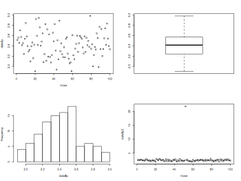
Measures of central tendency
x = c(rep(letters[1:5],3),rep(letters[6:10],4),rep(letters[11],8))

# Mode
xTable = table(x)[rev(order(table(x)))]
xTable[1]

# Other central tendency measures
# mu (mean): sum(x)/length(x)
# SS (sum of squares): sum((x-mean(x))^2)
# sigma^2: sum((x-mean(x))^2)/length(x)
# sigma: sqrt(sum((x-mean(x))^2)/length(x))

x = c(1,3,3,5)

# mean
sum(x)/length(x)
# SS
sum((x-mean(x))^2)
# sigma^2
sum((x-mean(x))^2)/length(x)
# sigma
sqrt(sum((x-mean(x))^2)/length(x))

library(psych)
describe(x)
Measures for shape of a distribution
# Skewness
# positive skew = scores bunched at low values and the tail pointing to high value
# negative skew = scores bunched at high values and the tail pointing to low value
# Kurtosis
# leptokurtic: heavy tails
# platykurtic: light tails

kurtosis = function(x) {
    m4 = mean((x-mean(x))^4)
    kurt = m4/(sd(x)^4)-3
    return(list(kurt=kurt))
}
skewness = function(x) {
    m3 = mean((x-mean(x))^3)
    skew = m3/(sd(x)^3)
    return(list(skew=skew))
}

x = rnorm(1000, mean=100, sd= 10)

kurtosis(x)
skewness(x)

library(psych)
describe(x)
Linear transformation of a distribution
# addition or subtraction with a constant C affects only mean (not dispersion)
# mean = mean + C (or mean - C)
# multiplication or division with a constant affects both mean and dispersion
# mean = mean / C
# variance = variance / C^2
# SD = SD / C

pdf("linearTransformation.pdf", width = 8, height = 6, onefile = TRUE, pointsize = 8)
par(mfrow=c(2,2))
x = c(3,4,4,5,6,7,8,8,9)
variance = function(x) { sum((x-mean(x))^2)/length(x) }
hist(x,main="Before transformation",col="gray75")
transformed_x = x - mean(x)
hist(transformed_x,main="Transformation to set the mean 0",col="gray75")
transformed_x = transformed_x/sqrt(variance(x))
hist(transformed_x,main="Transformation to set the SD to 1",col="gray75")
dev.off()
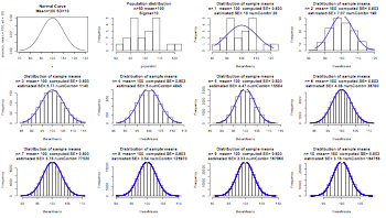
Standardization (z-score)
# z = (x-mu)/sigma
# use random numbers with mean 100 and sigma 10
temp <- rnorm(20)
sigma <- function(x){
	sqrt(sum((temp-mean(temp))^2)/length(temp))
}

# adjusting population mean to 100 and sigma to 10
population <- 100+10*((temp-mean(temp))/sigma(temp))
length(population) # 20
sigma(population) # 10
mean(population) # 100
# show the data
population

par(mfrow=c(3,4))
range <- c(70, 130)
x <- seq(min(range), max(range), len=200)
plot(x, dnorm(x, mean=100, sd=10), type="l", main="Normal Curve\nMean=100 SD=10")
x <- seq(90, 110, len=100)
y <- dnorm(x, mean=100, sd=10)
hist(population,main="Population distribution\nn=50 mean=100\nSigma=10")
for (i in seq(1,10,1)){
	# choosing i samples
	combinations <- combn(population, i)
	numComb <- length(combinations[1,])
	theseMeans <- apply(combinations,2,mean)
	thisMean <- mean(theseMeans)
	thisSE <- sigma(theseMeans)
	estimatedSE <- 10/sqrt(i)
	h <- hist(theseMeans,main=paste("Distribution of sample means\n","n=",i,
		" mean=",format(thisMean,digit=3)," computed SE=",format(thisSE,digit=3),
		"\n","estimated SE=",format(estimatedSE,digit=3),"numComb=",numComb))
	xfit<-seq(min(theseMeans),max(theseMeans),length=numComb)
	yfit<-dnorm(xfit,mean=mean(theseMeans),sd=sd(theseMeans))
	yfit <- yfit*diff(h$mids[1:2])*length(theseMeans)
	lines(xfit, yfit, col="blue", lwd=2)
}
par(mfrow=c(1,1))
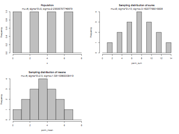
Sampling distributions
variance = function(x) { sum((x-mean(x))^2)/length(x) }

pdf("centralLimitTheorem.pdf", width = 8, height = 6, onefile = TRUE, pointsize = 8)
par(mfrow=c(2,2))

x = c(1,3,5,7)
hist(x,breaks=seq(0,8,1),col="gray75",main="Population")
mtext(paste("mu=",mean(x),"; ","sigma^2=",variance(x),"; ", "sigma=",sqrt(variance(x)),sep=""))
library(gtools)
# permutation and combination
# n: size of source, r: size of target
# number of permutations: n!/(n-r)!
# number of combinations: n!/(r!*(n-r)!)
sample_size = 2
perm = permutations(length(x),sample_size,x,repeats.allowed=TRUE)
perm_sum = apply(perm,1,sum)    # get sums of permutations
hist(perm_sum,breaks=seq(0,14,1),col="gray75",main="Sampling distribution of sums")
mtext(paste("mu=",mean(perm_sum),"; ","sigma^2=",variance(perm_sum),"; ", "sigma=",sqrt(variance(perm_sum)),sep=""))
perm_mean = perm_sum/sample_size
hist(perm_mean,breaks=seq(0,8,1),col="gray75",main="Sampling distribution of means")
mtext(paste("mu=",mean(perm_mean),"; ","sigma^2=",variance(perm_mean),"; ", "sigma=",sqrt(variance(perm_mean)),sep=""))

par(mfrow=c(1,1))
dev.off()
Built-in distributions
| Beta | beta | Log-normal | lnorm |
| Binomial | binom | Negative Binomial | nbinom |
| Cauchy | cauchy | Normal | rnom |
| Chisquare | chisq | Poisson | pois |
| Exponental | exp | Student t | t |
| Fisher F | f | Uniform | unif |
| Gamma | gamma | Tukey | tukey |
| Geometric | geom | Weibull | weib |
| Hypergeometric | hyper | Wilcoxon | wilcox |
| Logistic | logis | - | - |
| name | description | usage |
| dname() | density or probability function | dnorm(0) 1/ sqrt(2*pi); dnorm(1) exp(-1/2)/ sqrt(2*pi); dnorm(1) == 1/ sqrt(2*pi*exp(1)) |
| pname() | cumulative density function | pnorm(-1.63)=0.05155 (the area under the standard normal curve to the left of -1.63) |
| qname() | quantile function | qnorm(0.9)=1.2815 (1.2815 is the 90th percentile of the standard normal distribution) |
| rname() | drandam deviates | rnorm(100,mean=50,sd=10) (generates 100 random deviates from a normal distribution with the define parameters) |
# Probability distributions in R from
# http://www.statmethods.net/advgraphs/probability.html
pnorm(-2.58)
pnorm(-1.63)
pnorm(1.63)
pnorm(2.58)

qnorm(0.005)
qnorm(0.025)
qnorm(0.975)
qnorm(0.995)
Some applications
# mu = 100, sigma = 15, select one individual who is larger than 118
mu = 100; sigma = 15; n = 1
se = sigma/sqrt(n)
z = (118-100)/se
1 - pnorm(z)

# mu = 100, sigma = 15, select one individual between 79 and 94
mu = 100; sigma = 15; n = 1
se = sigma/sqrt(n)
z_low = (79-100)/se
z_high = (94-100)/se
pnorm(z_high) - pnorm(z_low)

# mu = 100, sigma = 15, select 4 samples whose mean is larger than 118
mu = 100; sigma = 15; n = 4
se = sigma/sqrt(n)
# z-score for sample means
z = (118-100)/se
1 - pnorm(z)

# mu = 100, sigma = 15, conf interval of 36 samples with 95% confidence
mu = 100; sigma = 15; n = 36
se = sigma/sqrt(n)
z_low = qnorm(0.025)
z_high = qnorm(0.975)
# x = z*se + mu
z_low*se + mu
z_high*se + mu
One-sample t-test (W2)
Assumptions of t-test
- variable type: the responce variable is continuous and the predictor variable is categorical
- independence of sampling: sampling is independent each other
- normality: the distribution of the population is normally distributed
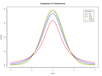
Demonstrating t-distributions
###########
# Normal and t-distribution
###########
# From Quick-R http://www.statmethods.net
# Display the Student's t distributions with various
# degrees of freedom and compare to the normal distribution

pdf("distributionPlots.pdf", width = 8, height = 6, onefile = TRUE,           pointsize = 8)
x = seq(-4, 4, length=100)
hx = dnorm(x)
degf = c(1, 3, 8, 30)
colors = c("red", "blue", "darkgreen", "gold", "black")
labels = c("df=1", "df=3", "df=8", "df=30", "normal")

plot(x, hx, type="l", lty=2, xlab="x value", ylab="Density", main="Comparison of t Distributions")
for (i in 1:4){
    lines(x, dt(x,degf[i]), lwd=2, col=colors[i])
}
legend("topright", inset=.05, title="Distributions", labels, lwd=2, lty=c(1, 1, 1, 1, 2), col=colors)
dev.off()
Hypothesis test of mu
# mu = 50, sigma = 10, n = 10, x_bar = 58
mu = 50; sigma = 10; n = 10; x_bar = 58
se = sigma/sqrt(n)
z_low = qnorm(0.025)
z_high = qnorm(0.975)
# x = x_bar + z*se
x_bar + z_low*se
x_bar + z_high*se
Biased and unbiased estimations of variance
# s2 = sum((x-mean(x))^2)/(length(x)-1)
# s = sqrt(s2)
# se_xbar = s/sqrt(length(n))

s2 = function(x) { sum((x-mean(x))^2)/(length(x)-1) }
variance = function(x) { sum((x-mean(x))^2)/length(x) }

x = c(2,4,6,8)
library(gtools)
sample_size = 2
perm = permutations(length(x),sample_size,x,repeats.allowed=TRUE)

thisData = cbind(perm,apply(perm,1,s2),apply(perm,1,variance))
thisData = as.data.frame(thisData)
colnames(thisData) = c("X_1","X_2","sample_var","population_var")
thisData
Critical values of t
dfs = c(5,10,20,40,80,1000)

func1 = function(x) { qt(0.975,x) }
func2 = function(x) { qt(0.995,x) }

thisData = cbind(t(dfs),apply(dfs,1,func1),apply(dfs,1,func2))
thisData = as.data.frame(thisData)
colnames(thisData) = c("df","alpha_0.05","alpha_0.01")
thisData
Estimating mu with sample variance
# mu = 50, n = 100, x_bar = 54, s = 19. What is the conf interval of mu?
mu = 50; n = 100; x_bar = 54; s = 19
se = s/sqrt(n)
x_bar + qt(.975,n-1)*se
x_bar - qt(.975,n-1)*se
Correlation and Regression (W3)
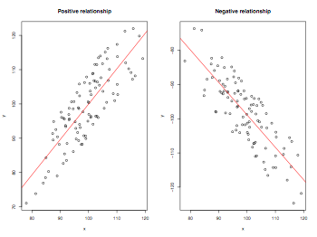
Positive and negative correlations
pdf("correlations.pdf", width = 8, height = 6, onefile = TRUE, pointsize = 8)
par(mfrow=c(1,2))
x = rnorm(100,mean=100,sd=10)
y = jitter(x, factor=10, amount = 10)
plot(x,y,main="Positive relationship")
abline(lm(y~x),col="red")

y = jitter(-x, factor=10, amount = 10)
plot(x,y,main="Negative relationship")
abline(lm(y~x),col="red")
dev.off()
Demonstration of correlation r (hand calculation)
# covariance: sum((x-mean(x))*(y-mean(y))/(n_x + n_y - 1)
# s_x = sqrt(sum((x-mean(x))**2)/(n_x-1))     # or sd(x)
# s_y = sqrt(sum((y-mean(y))**2)/(n_y-1))     # or sd(y)
# r = cov/(s_x * s_y)

x = seq(1,6)
y = c(.440,.515,.550,.575,.605,.615)
thisData = cbind(x,y,x-mean(x),y-mean(y),(x-mean(x))*(y-mean(y)))
thisdata = as.data.frame(thisData)
colnames(thisData) = c("setsize","RT","x-xbar","y-ybar","(x-xbar)(y-ybar)")

cov = sum((x-mean(x))*(y-mean(y)))/(length(x)-1)
s_x = sqrt(sum((x-mean(x))**2)/(length(x)-1))     # or sd(x)
s_y = sqrt(sum((y-mean(y))**2)/(length(y)-1))     # or sd(y)

r = cov/(s_x * s_y)
cov; s_x; s_y; r
Demonstration of correlation r (built-in function)
x = seq(1,6)
y = c(.440,.515,.550,.575,.605,.615)
cor.test(x,y)

library(psych)
describe(cbind(x,y))
Demonstration of regression (built-in function)
x = seq(1,6)
y = c(.440,.515,.550,.575,.605,.615)

fit = lm(y~x)
summary(fit)

library(psych)
describe(cbind(x,y))
Producing correlation matrix
thisData = as.data.frame(seq(1:6))
for (i in 1:7) {
	x = sort(rnorm(1000,mean=100,sd=i))
	thisData[i] <- sample(x, 6)
}

# printing correlation matrix
cor(thisData)

# computing a p-value for one correlation
cor.test(thisData[,1],thisData[,2])

# modified from the formula posted on R-help by Bill Venables
cor.prob <- function(X, dfr = nrow(X) - 2) {
	R <- cor(X)
	above <- row(R) < col(R)
	below <- row(R) > col(R)
	r2 <- R[above]^2
	Fstat <- r2 * dfr / (1 - r2)
	R[above] <- 1 - pf(Fstat, 1, dfr)
	R[below] <- 0
	R
}
cor.prob(thisData)
Comparing two means (t-test) (W4)
Assumptions of t-test
- variable type: the responce variable is continuous and the predictor variable is categorical
- independence of sampling: sampling is independent each other
- normality: the distribution of the population is normally distributed
- the variances of the populations to be compared are equal
Dependent t-test (hand calculation)
x = rbind(c("A",550,510),c("B",1030,980),c("C",760,770), c("D",600,600),c("E",940,870),c("F",820,760))
x = as.data.frame(x)
colnames(x) = c("Subject","Unprimed","Primed")
x$Primed = as.double(as.character(x$Primed))
x$Unprimed = as.double(as.character(x$Unprimed))

x$Difference = x$Unprimed - x$Primed
sum(x$Difference)
mean(x$Difference)
sd(x$Difference)
se = sd(x$Difference)/sqrt(length(x$Difference))
qt(0.975,5)                # critical t-value for alpha=0.05 df=5
t = (mean(x$Difference)-0)/se
df = length(x$Differenc)-1
dt(t,df)
Dependent t-test (built-in function)
x = c(550,1030,760,600,940,820)
y = c(510,980,770,600,870,760)

t.test(x,y,paired=TRUE)

library(psych)
describe(cbind(x,y))
Problems with repeated-measures (within-subjects) research designs
- Order effects: Subject may improve or become fatigued over time
- counter balancing (half the subjects get A first and B; the other half the reverse order)
- intermixing (multiple trials are randomly interleaved (ABBABABBAAAB...)
- Carryover effects: the effect of the first treatment may effect the second treatment
- Difficulty in matching: Mutually exclusive subject selection categories are difficult to match pairs
Variance Sum Law
# The variance of the sum or difference of two independent variables is equal to the sum of their variances
# var(x_bar1 - x_bar2) = s_1^2/n_1 + s_22/n_2
# se(x_bar1 - x_bar2 )= sqrt(s_1^2/n_1 + s_22/n_2)
Comparison between independent and dependent t-tests
x = c(550,1030,760,600,940,820)
y = c(510,980,770,600,870,760)

t.test(x,y,paired=FALSE)
t.test(x,y,paired=TRUE)

library(psych)
describe(cbind(x,y))
Independent t-test = point-biserial correlation
# regression approach to t-test
# Independent t-test = point-biserial correlation

x = c(rep(0,6),rep(1,6))
y = c(55,73,76,66,72,81,71,93,77,89,101,97)

summary(lm(y~x))

thisData = as.data.frame(cbind(x,y))
t.test(thisData[thisData$x  0,"y"],thisData[thisData$x  1,"y"],var.equal=TRUE)
Graphics for t-test
data = read.table("das.txt",header=TRUE)

pdf("t-testGrahpics.pdf", width = 8, height = 6, onefile = TRUE, pointsize = 8)
par(mfrow=c(2,2))
plot(data$y)
boxplot(data$y)
hist(data$y,main="")
data$y2 = data$y
data$y2[52] = 21.75
plot(data$y2)
dev.off()
Test for normality (Shapiro test)
# the Shapiro test for testing whether the data come form a normal distribution
x = exp(rnorm(30))
shapiro.test(x)
One-sample t-test
y = c(1,-2,2,1,-4,5,-8,-5,2,5,6)

t.test(y,mu=2)
Independent two-group t-test (numeric variable and grouping factor)
# make a dummy data set
x = c(rep(1,8),rep(2,5))
levels(x) = c("A","B")
y = c(7,5,6,8,4,5,4,6,3,5,4,6,2)
thisData = cbind(x,y)
thisData = as.data.frame(thisData)
thisData$x = factor(thisData$x)
levels(thisData$x) = c("A","B")

t.test(thisData$y~thisData$x)
Independent two-group t-test (two numeric vectors)
x = c(7,5,6,8,4,5,4,6)
y = c(3,5,4,6,2)

t.test(x,y)
Paired/Dependent t-test (two numeric vectors)
x = c(4,5,6,4,5,6,6,4)
y = c(2,1,4,5,6,9,2,2)

t.test(x,y,paired=TRUE)
More correlation (W5)
Assumptions of Correlations
- variable type: both variables are continuous
- normality: the distribution of both variables are approximatly normal
- linearity: the relationship between two variables is, in reality, linear
- homoscedasticity: the variance of the error term should be constant
Comparing two correlations
# comparing two correlation coefficients
# fon.hum.uva.nl/Service/Statistics/Two_Correlations.html
compcorr = function(n1, r1, n2, r2){
    # compare two correlation coefficients
    # return difference and p-value as list(diff, pval)
    # Fisher Z-transform
    # Zf = 1/2 * ln((1+R)/(1-R))
    zf1 = 0.5*log((1 + r1)/(1 - r1))
    zf2 = 0.5*log((1 + r2)/(1 - r2))

    # difference
    # z = (Zf1 - Zf2) / SQRT( 1/(N1-3) + 1/(N2-3) )
    dz = (zf1 - zf2)/sqrt(1/(n1 - 3) + (1/(n2 - 3)))

    # p-value (two-tails)
    pv = 1 - pnorm(abs(dz))
    return(list(z1=zf1,z2=zf2,diff=dz, pval=pv))
}

# r_male = -.506, n_male = 52, r_female = -.381, n_female = 51
r_male = -.506; n_male = 52; r_female = -.381; n_female = 51

compcorr(n_male,r_male,n_female,r_female)
Partial and semi-partial correlations
# partial correlation
# remove the effect of one predictor from other predictors and the outcome
# (correlation while controlling for another variable, partialing out another
# variable, or keeping another variable constant)
partialCor = function(predictor_1,dependent_y,predictor_2){
# partialing out the effect of predictor_2 from predictor_1 and dependent_y
# r_xy.z = (r_xy - r_xz*r_yz)/(sqrt((1-r_xz**2)*(1-r_yz**2)))
r_xy = cor(predictor_1,dependent_y)
r_xz = cor(predictor_1,predictor_2)
r_yz = cor(dependent_y,predictor_2)
pc <- (r_xy - r_xz*r_yz)/(sqrt((1-r_xz**2)*(1-r_yz**2)))
return(list(partialCorrelation=pc))
}
# computing partCor with residuals -- this also tests significance
partialCor2 <- function(x, y, z) {
return(cor.test(lm(x~z)$resid,lm(y~z)$resid));
}
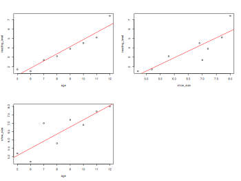
child = rep(letters[1:8])
shoe_size = c(5.2,4.7,7,5.8,7.2,6.9,7.7,8)
reading_level = c(1.7,1.5,2.7,3.1,3.9,4.5,5.1,7.4)
age = c(5,6,7,8,9,10,11,12)
library(Hmisc)
rcorr(cbind(reading_level,age,shoe_size))
pdf("partialCorrelation.pdf", width = 8, height = 6, onefile = TRUE, pointsize = 8)
par(mfrow=c(2,2))
plot(age,reading_level)
abline(lm(reading_level~age),col="red")
plot(shoe_size,reading_level)
abline(lm(reading_level~shoe_size),col="red")
plot(age,shoe_size)
abline(lm(shoe_size~age),col="red")
dev.off()
partialCor(reading_level,shoe_size,age)
res_shoe.age = lm(shoe_size~age)$residuals
res_read.age = lm(reading_level~age)$residuals
cor.test(res_shoe.age,res_read.age)
# semi-partial correlation
semipartialCor = function(pred_1,y,pred_2){
# partialing out the effect of 2 from 1 (but not from y)
# r_y1.2 = (r_1y - r_2y*r_12)/sqrt((1-r_2y**2)*(1-r_12**2))
sp <- (cor(pred_1,y) - cor(pred_2,y)*cor(pred_1,pred_2))/ sqrt((1-cor(pred_1,pred_2)**2))
return(list(semiPartialCorrelation=sp))
}
semipartialCor(reading_level,shoe_size,age)
Multiple regressions (W6)
Assumptions of Multiple Regression
- variable type: Outcome is continuous and predictors are continuous/dichotomous
- non-zero variance: Predictors must not have zero variance
- linearity: The relationship of the model is, in reality, linear
- independence: All values of the outcome should be independent
- no multicollinearity: Predictors must not be highly correlated (Tolerance > 0.2; VIF < 10)
- homoscedasticity: The variance of the error term should be constant
- independent errors: The error terms should be uncorrelated (Durbin-Watson test = 2)
- normally-distributed errors
Computing SSs (built-in functions)
thisData = read.table("mtcars.txt",header=TRUE)

# computing SSs
SSY.manual = sum((thisData$disp - mean(thisData$disp))^2)
SSY.formula = deviance(lm(disp~1, data=thisData))
SSE = deviance(lm(disp ~ cyl, data=thisData))
SSY.manual; SSY.formula; SSE

# linear model (regression) with intercept
fit1 = lm(disp ~ cyl, data=thisData)
summary(fit1)

# linear model (regression) without intercept
fit2 = lm(disp ~ cyl - 1, data=thisData)
summary(fit2)
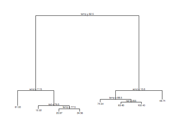
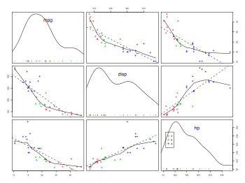
Plots for multiple regression
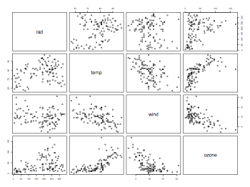
ozone.pollution = read.table("ozone.data.txt",header=TRUE)
attach(ozone.pollution)
names(ozone.pollution)
pdf("ozonePollutionPairsScatterplot.pdf", width = 8, height = 6, onefile = TRUE, pointsize = 8)
pairs(ozone.pollution, panetl=panel.smooth)
dev.off()
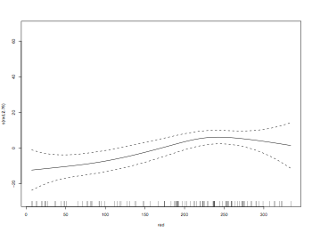
library(mgcv)
par(mfrow=c(2,2))
pdf("ozonePollutionModelPlot.pdf", width = 8, height = 6, onefile = TRUE, pointsize = 8)
model = gam(ozone ~ s(rad)+s(temp)+s(wind))
plot(model)
dev.off()
par(mfrow=c(1,1))
library(tree)
pdf("ozonePollutionTreePlot.pdf", width = 8, height = 6, onefile = TRUE, pointsize = 8)
model = tree(ozone ~ .,data = ozone.pollution)
plot(model)
text(model)
dev.off()
B slopes
# Standardized regression equation (cf. semi-partial correlation)
# B_1 = (r_1y-r_2y*r_12)/(1-r_12^2)
# B_2 = (r_2y-r_1y*r_12)/(1-r_12^2)
# R = sqrt(B_1*r_1y + B_2*r_2y)

# correlations of pred1, pred2, and predicted var y
# r_1y = .4, r_2y = .3, r_12 = .2
r_1y = .4; r_2y = .3; r_12 = .2
B_1 = (r_1y-r_2y*r_12)/(1-r_12^2)
B_2 = (r_2y-r_1y*r_12)/(1-r_12^2)
B_1; B_2
R = sqrt(B_1*r_1y + B_2*r_2y)
R; R^2

# correlations of pred1, pred2, and predicted var y
# r_1y = .4, r_2y = .3, r_12 = .75
r_1y = .4; r_2y = .3; r_12 = .75
B_1 = (r_1y-r_2y*r_12)/(1-r_12^2)
B_2 = (r_2y-r_1y*r_12)/(1-r_12^2)
B_1; B_2
Complementarity and Suppression
# Complementarity
# Predictors are positively correlated with Y but negatively correlated
# with each other
r_1y = .4; r_2y = .3; r_12 = -.2
B_1 = (r_1y-r_2y*r_12)/(1-r_12^2)
B_2 = (r_2y-r_1y*r_12)/(1-r_12^2)
B_1; B_2
R = sqrt(B_1*r_1y + B_2*r_2y)
R; R^2

# Suppression
# pred2 is not correlated with Y, but is correlated with pred1.
# When pred2 is in the model, semi-partial correlation is higher
# than the zero-order correlation
r_1y = .4; r_2y = 0; r_12 = .5
B_1 = (r_1y-r_2y*r_12)/(1-r_12^2)
B_2 = (r_2y-r_1y*r_12)/(1-r_12^2)
B_1; B_2
Dummy data (mtcar)
# mpg: Miles/(US) gallon; cyl: Number of cylinders; disp: Displacement (cu.in.)
# hp: Gross horsepower; drat: Rear axle ratio; wt: Weight (lb/1000)
# qsec: 1/4 mile time; vs: V/S; am: Trans (0 = auto, 1 = man)
# gear: Number of forward gears; carb: Number of carburetors
thisData = read.table("mtcars.txt",header=TRUE)
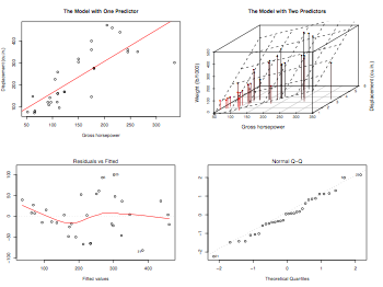
Data visualization
thisData = read.table("mtcars.txt",header=TRUE)
attach(thisData)
pdf("multipleRegressionGraphics.pdf", width = 8, height = 6, onefile = TRUE, pointsize = 8)
par(mfrow=c(2,2))
plot(disp~hp,main="The Model with One Predictor",ylab="Displacement (cu.in.)" ,xlab="Gross horsepower")
abline(lm(disp~hp),col="red")

library(scatterplot3d)
s3d = scatterplot3d(hp,wt,disp, pch=16, highlight.3d=TRUE, type="h",
            main="The Model with Two Predictors",ylab="Displacement (cu.in.)",
            xlab="Gross horsepower",zlab="Weight (lb/1000)")
fit = lm(disp~hp+wt)
s3d$plane3d(fit)
plot(fit)
dev.off()
detach()
Methods of multiple regression
# hierarchical: known predictors are entered into the regression model first
#               then, new predictors are entered in a separate block
# forced entry: all variables are entered into the model simultaneously
# stepwise    : variables are entered into the model based on mathematical criteria

thisData = read.table("mtcars.txt",header=TRUE)
attach(thisData)

# hierarchical model
cor(thisData)

fit1 = lm(disp ~ mpg + cyl + hp + wt + gear, data=thisData)
fit2 = lm(disp ~ mpg + cyl + hp, data=thisData)
fit3 = lm(disp ~ hp, data=thisData)
anova(fit1, fit2, fit3)

coefficients(fit1)           # model coefficients
confint(fit1, level=0.95)    # CIs for model parameters
fit1ted(fit1)                # predicted values
residuals(fit1)              # residuals
anova(fit1)                  # anova table
vcov(fit1)                   # covariance matrix for model parameters
influence(fit1)              # regression diagnostics

# Stepwise Regression
library(MASS)
fit4 = lm(disp ~ mpg + cyl + hp + drat + wt + qsec + gear , data=thisData)
step = stepAIC(fit4, direction="both")
step$anova
step = stepAIC(fit4, direction="forward")
step$anova
step = stepAIC(fit4, direction="backward")
step$anova
Some diagnostic tests for multiple regression
- Identifying outlifers from the case summaries
- no more than 5% of cases are above 2 SD
- no more than 1% of cases are above 2.5 SD
- any case is more than 3 SD
- Cook's distance larger than 1 causes for concern
- Big Leverage values cause for concern
- Mahalanobis distance (value above 25/15) causes for concern
- CVR (covariance ratio) not close to 1 causes for concern
Effect size (W7)
- Unstandardized (absolute) effect size
- "If the units of measurement are meaningful on a practica llevel (e.g., number of cigaretts smoked per day), then we usually perfer an unstandarized measure (regression coefficient or mean difference) to a standardized measure (r or d)" (Wilkinson et al., 1999, p.599)
- r-family: r = variance explained / total variance
- simple regression: r/r^2
- multiple regression: R/R^2
- t-test: r=sqrt(t^2/(t^2+df))
- ANOVA: etha^2/omega^2
- chi-square: odd ratio
- Interpretation: r=.10 (small effect; explains 1% of variance), r=.3 (medium effect), r=.5 (large effect)
- d-family: variance explained / variance not explained
- d = (mu_1 - mu_2)/ sigma (standardized mean difference)
- Interpretation: d=.20 (small effect; separation of .3 sd), d=.5 (medium effect), d=.8 (large effect)
- d is not bounded the way that r is, so d can be larger than 1
- Alpha (the probability of a Type I error)
- Type I error: rejecting null hypothesis that is true
- Beta (the probability of a Type II error)
- Type II error: not detecting a real difference / failing to reject null hypothesis that is false
- Power (1-beta): detecting a real difference / rejecting null hypothesis that is false
- To increase power
- make alpha larger
- use a 1-tailed test instread of 2-tailed
- increase the effect size (e.g., use a larger difference between DV)
- decrease the variabilty of the data
- increase the sample size
Power analysis
# tw-sample (independent groups) t-test
# effect size d = 0.4, alpha = .05, two-tailed, expected t = 2.80 (Power = 0.8)
# how many subjects are required?
library(pwr)
pwr.t.test(n=NULL,d=0.4,sig.level=.05,power=0.8,type="two.sample",alternative="two.sided")
pwr.t.test(n=NULL,d=0.4,sig.level=.05,power=0.8,type="paired",alternative="two.sided")
One-way ANOVA (W8)
Levene's test (of equity of variance)
# SPSS uses the Levene's test as default test for testing the constancy of variance
levene.test = function(y, group) {
    meds = tapply(y, group, median, na.rm=TRUE)
    resp = abs(y - meds[group])
    table = anova(lm(resp ~ group, na.action=na.omit))
    row.names(table)[2] = " "
    cat("Levene's Test for Homogeneity of Variance\n\n")
    table[,c(1,4,5)]
}

# make a dummy data set
x = c(rep(1,5),rep(2,3),rep(3,5))
y = c(7,5,6,8,4,5,4,6,3,5,4,6,2)
thisData = cbind(x,y)
colnames(thisData) = c("group","score")
thisData = as.data.frame(thisData)
thisData$group = as.factor(thisData$group)

# do one-way ANOVA
summary(aov(score~group,data=thisData))       # with aov()
summary(lm(score~group,data=thisData))        # with lm()
anova(lm(score~group,data=thisData))          # anova table
summary(lm(score~group-1,data=thisData))      # with lm() without intercept
anova(lm(score~group-1,data=thisData))        # anova table

# do the Levene's test
levene.test(thisData$score,thisData$group)
Planned comparisons and post-hoc test (W9)
Planned comparisons
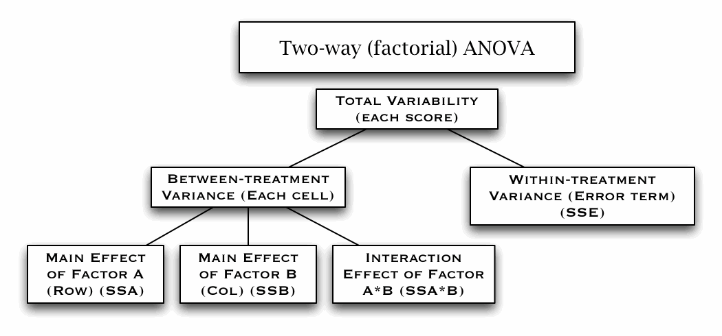
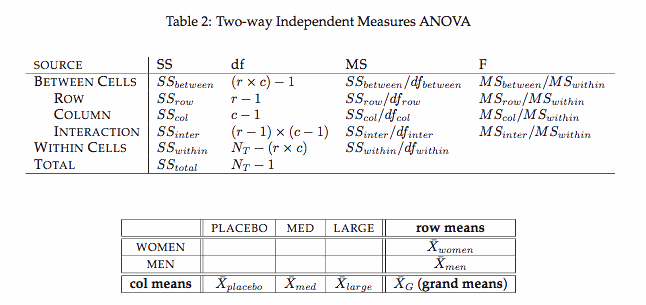
Two-way Factorial ANOVA (W10)
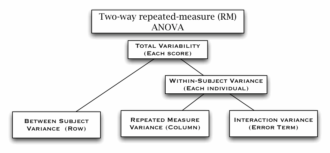
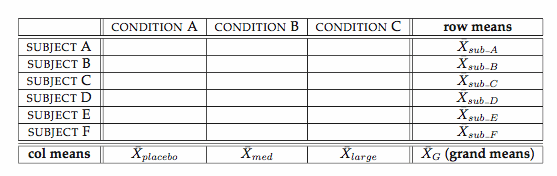
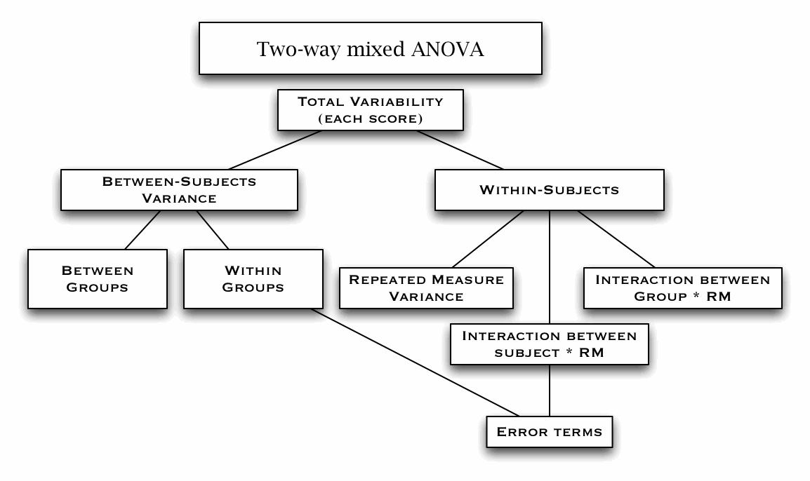
Two-way Repeated Measure ANOVA (W11)
Common errors!
# Don't forget to check the data when you transform the format (with melt() or apply()).
# Fix the factor variables with as.factor() if necessary. Set sum-to-zero so that the
# results are comparable with other statistical software such as SPSS

options(contrasts=c("contr.sum","contr.poly"))
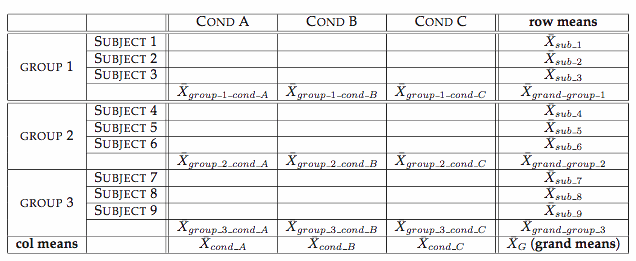
Data format for RM measures
# The data format for RM measures in R is different from that for SPSS.
# In R (and most other statistical software), the RM measure should be one of the factors.
# In other words, each line represents one data point.

   gender variable value
1    male    early     4
2    male    early    10
3    male    early     5
4  female    early     8
5  female    early     2
6    male      mid     6
7    male      mid     9
8    male      mid     4
9  female      mid     6
10 female      mid     2
11   male     late     2
12   male     late     8
13   male     late     3
14 female     late     7
15 female     late     2

# In SPSS, the RM measure is represented by multiple data points in one row.
# In other words, within-factors are represented by the row.

  early mid late gender
1     4   6    2   male
2    10   9    8   male
3     5   4    3   male
4     8   6    7 female
5     2   2    2 female

# Even in SPSS, the data format similar to that for R is required for a more complex
# analyses (e.g., one that involves more than two within factors). In such a case,
# dummy coding is used (thus, the data format is almost identical to that for R).
# Use melt() in the reshape package to transform the data format for SPSS to that for R.
Calculating SS (hand-calculation)
# SS_total = SS_bet_sub + SS_within_sub

# make a dummy data set
thisData = rbind(c(4,6,2),c(10,9,8),c(5,4,3),c(8,6,7),c(2,2,2))
thisData = as.data.frame(thisData)
colnames(thisData) = c("early","mid","late")

# SS from each score (total variability)
# sum((score - grand_mean)^2)
grand_mean = mean(mean(thisData))
sum((thisData - grand_mean)^2)

# SS from row means (within-subject variability)
# sum((score-row_mean)^2)
row_mean = apply(thisData,1,mean)
sum((thisData-row_mean)^2)

# between-subject variability
# sum(n*(row_mean-grand_mean)^2)
grand_mean = mean(mean(thisData))
row_mean = apply(thisData,1,mean)
n = length(thisData[1,])
sum(n*(row_mean-grand_mean)^2)

# col means (RM variability)
# sum(n*(col_mean-grand_mean)^2)
grand_mean = mean(mean(thisData))
col_mean = apply(thisData,2,mean)
n = length(thisData[,1])
sum(n*(col_mean-grand_mean)^2)
Field textbook Ch.13 Repeated-measure ANOVA (demo using R)
library(foreign); library(reshape); library(psych); library(nlme); library(car); library(ez); library(gplots)
thisData <- read.spss( "DiscoveryingStatsSPSS3/Bushtucker.sav", to.data.frame=TRUE)
summary(thisData)
describe(thisData) # p.474
## change to the sum-to-zero convention (cf. Type II and Type III sums of squares)
#default.contrast = options("contrasts")
#options(contrasts=c("contr.sum","contr.poly"))
# using Anova() in the car package
fit1 <- lm(as.matrix(thisData) ~ 1)
factors.thisData <- colnames(thisData)
fit1.aov <- Anova(fit1, idata=data.frame(factors.thisData), idesign = ~factors.thisData, type="III")
summary(fit1.aov)
# reformatting the data structure
thisData$subject <- as.factor(rownames(thisData))
thisData.molten <- melt(thisData)
# aov() and lme() do not support Mauchly test and Thurkey HSD
fit2 <- lme(value ~ variable, random = ~1|subject/variable, data=thisData.molten)
summary(fit2)
fit3 <- aov(value ~ variable + Error(subject/variable), data=thisData.molten)
summary(fit3)
# or use ezANOVA()
fit4 <- ezANOVA(data=thisData.molten, dv=.(value), wid=.(subject), within=.(variable))
fit4
# new data (pp.483-)
thisData <- read.spss( "DiscoveryingStatsSPSS3/Attitude.sav", to.data.frame=TRUE)
describe(thisData)
thisData$subject <- as.factor(rownames(thisData))
thisData.molten <- melt(thisData)
thisData.molten[grep("beer",thisData.molten$variable),"drink"] <- "beer"
thisData.molten[grep("wine",thisData.molten$variable),"drink"] <- "wine"
thisData.molten[grep("water",thisData.molten$variable),"drink"] <- "water"
thisData.molten[grep("pos",thisData.molten$variable),"image"] <- "sexy"
thisData.molten[grep("neg",thisData.molten$variable),"image"] <- "corpse"
thisData.molten[grep("neut?",thisData.molten$variable),"image"] <- "person in armchair"
thisData.molten$drink <- factor(thisData.molten$drink,levels=c("beer","wine","water"))
thisData.molten$image <- factor(thisData.molten$image,levels=c("sexy","corpse","person in armchair"))
fit5 <- ezANOVA(data=thisData.molten, dv=.(value), wid=.(subject), within=.(drink,image))
fit5
color = c("lightyellow","lightblue","lightgreen")
pdf("RMANOVABarchart.pdf", width = 10, height = 8, onefile = TRUE, pointsize = 8)
thisData.mean = tapply(thisData.molten$value,thisData.molten$drink,mean)
thisData.sd = tapply(thisData.molten$value,thisData.molten$drink,sd)
thisData.n = tapply(thisData.molten$value,thisData.molten$drink,length)
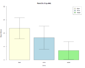
barplot2(thisData.mean,ylim=c(0,20),beside=TRUE,
main="Field Ch.13 (p.494)",
ylab="Mean Attitude",xlab="Drink",col=color,
ci.l=thisData.mean+((thisData.sd/sqrt(thisData.n))*qt(0.025,df=(thisData.n-1))),
ci.u=thisData.mean+((thisData.sd/sqrt(thisData.n))*qt(0.975,df=(thisData.n-1))),
plot.ci=TRUE)
labs = c("Beer","Wine","Water")
legend("topright",labs,fill=color)
dev.off()
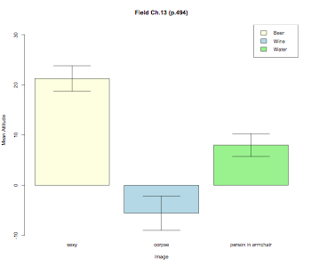
pdf("RMANOVABarchart2.pdf", width = 10, height = 8, onefile = TRUE, pointsize = 8)
thisData.mean = tapply(thisData.molten$value,thisData.molten$image,mean)
thisData.sd = tapply(thisData.molten$value,thisData.molten$image,sd)
thisData.n = tapply(thisData.molten$value,thisData.molten$image,length)
barplot2(thisData.mean,ylim=c(-10,32),beside=TRUE,
main="Field Ch.13 (p.494)",
ylab="Mean Attitude",xlab="Image",col=color,
ci.l=thisData.mean+((thisData.sd/sqrt(thisData.n))*qt(0.025,df=(thisData.n-1))),
ci.u=thisData.mean+((thisData.sd/sqrt(thisData.n))*qt(0.975,df=(thisData.n-1))),
plot.ci=TRUE)
labs = c("Beer","Wine","Water")
legend("topright",labs,fill=color)
dev.off()
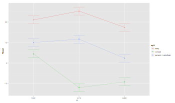
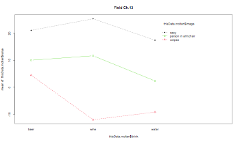
pdf("RMANOVABarchart3.pdf", width = 10, height = 8, onefile = TRUE, pointsize = 8)
ezPlot(data=thisData.molten, dv=.(value), wid=.(subject), within=.(drink,image), x=.(drink), split=.(image))
interaction.plot(thisData.molten$drink,thisData.molten$image,thisData.molten$value, type="b", col=c(1:3), pch=c(18,24,22), main="Field Ch.13")
dev.off()
Repeated-measure ANOVA (one-way; built-in function)
# make a dummy data set
thisData = rbind(c(4,6,2),c(10,9,8),c(5,4,3),c(8,6,7),c(2,2,2))
thisData = as.data.frame(thisData)
colnames(thisData) = c("early","mid","late")

library(reshape)
# make a new col to keep the subject id
temp = cbind(thisData,as.factor(rownames(thisData)))
colnames(temp) = c(colnames(thisData),"subject")
thisData = melt(temp,id=c("subject"))

# conduct one-way RM ANOVA
fit = aov(value~variable + Error(subject/variable),data=thisData)
summary(fit)
Repeated-measure ANOVA (one-way; with follow-up tests)
# read data from local disk
thisData =  read.table("Pitt_Shoaf3.txt", header=TRUE)

# aggregate the data (i.e., collapsing the 'overlap' factor)
aggregatedData = aggregate(thisData$rt,list(thisData$subj,thisData$position),mean)
colnames(aggregatedData) = c("subj","position","rt")

library(psych)
by(aggregatedData$rt,list(aggregatedData$position),describe)

# do one-way RM ANOVA with aov()
# there is no built-in Sphericity test and post-hoc test (TurkeyHSD)
fit = aov(rt ~ position + Error(subj/position), data=aggregatedData)
summary(fit)

# do one-way RM ANOVA with lme() in the nlme package
# there is no built-in Sphericity test and post-hoc test (TurkeyHSD)
require(nlme)
fit2 = lme(rt ~ position, random = ~1|subj, data=aggregatedData)
summary(fit2)
anova(fit2)

# do one-way RM ANOVA with lm()/mlm() (multivariate approach)
# See gribblelab.org/2009/03/09/repeated-measures-anova-using-r/
crossTabulatedData = xtabs(rt ~ subj + position, data=thisData)/2
crossTabulatedData

mlm1 = lm(crossTabulatedData ~ 1)

position = factor(colnames(crossTabulatedData))
mlm1.aov = Anova(mlm1, idata = data.frame(position), idesign = ~position, type="III")

summary(mlm1.aov, multivariate=FALSE)

# pairwise t-test
contrastD = crossTabulatedData[,1]-crossTabulatedData[,2]
t.test(contrastD)

contrastD = crossTabulatedData[,1]-crossTabulatedData[,3]
t.test(contrastD)

contrastD = crossTabulatedData[,2]-crossTabulatedData[,3]
t.test(contrastD)
Repeated-measure ANOVA (two-way)
# read data from local disk
thisData =  read.table("Pitt_Shoaf3.txt", header=TRUE)

# cross tabulate by two factors
crossTabulatedData = xtabs(rt ~ subj + position + overlap, data=thisData)

# SPSS requires a strange data format for two-way RM ANOVA
temp.threeOverlap = as.data.frame(crossTabulatedData[,,1])
temp.zeroOverlap = as.data.frame(crossTabulatedData[,,2])
colnames(temp.threeOverlap) = paste(colnames(temp.threeOverlap),"3",sep="_")
colnames(temp.zeroOverlap) = paste(colnames(temp.zeroOverlap),"0",sep="_")

data4SPSS = data.frame(temp.threeOverlap,temp.zeroOverlap,check.names=TRUE,       check.rows=TRUE)

library(psych)
describe(aggregatedData)

# do two-way factorial RM ANOVA with aov()
# there is no built-in Sphericity test and post-hoc test (TurkeyHSD)
fit = aov(rt ~ position*overlap + Error(subj/(position*overlap)), data=thisData)
summary(fit)

# how can I do two-way RM ANOVA with lme() in the nlme package?
Mixed-design ANOVA (W12)
Field textbook Ch.14 Mixed-design ANOVA (demo using R)
library(foreign)
library(reshape)
thisData <- read.spss( "DiscoveryingStatsSPSS3/LooksOrPersonalityGraphs.sav", to.data.frame=TRUE)
thisData.subset <- subset(thisData,!is.na(gender),c("gender","att_high","av_high","ug_high",
"att_some","av_some","ug_some","att_none","av_none","ug_none"))
thisData.subset$subject <- as.factor(rownames(thisData.subset))
newData <- melt(thisData.subset,c("subject","gender"))
newData$subject <- factor(newData$subject,levels=c(1:20))
newData[grep("_high",newData$variable),"charisma"] <- "high"
newData[grep("_some",newData$variable),"charisma"] <- "some"
newData[grep("_none",newData$variable),"charisma"] <- "dullard"
newData$charisma <- factor(newData$charisma,levels=c("high","some","dullard"))
newData[grep("att_",newData$variable),"looks"] <- "attractive"
newData[grep("av_",newData$variable),"looks"] <- "average"
newData[grep("ug_",newData$variable),"looks"] <- "ugly"
newData$looks <- factor(newData$looks,levels=c("attractive","average","ugly"))
colnames(newData)[4] <- "rate"
# this is wrong! Repeated measures are no taken into consideration.
# the DF is far larger than the actural subject size
model1 <- aov (rate~charisma*looks,data=newData)
summary(model1)
# exactly the same results as Field's book (pp.516-517)
ftable(tapply(newData$rate,list(newData$gender,newData$charisma,newData$looks),mean))
ftable(tapply(newData$rate,list(newData$gender,newData$charisma,newData$looks),sd))
ftable(tapply(newData$rate,list(newData$gender,newData$charisma,newData$looks),length))
model2 <- aov(rate~gender*charisma*looks+Error(subject/charisma*looks),data=newData)
summary(model2)
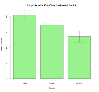
# bar plot
num <- length(unique(newData$subject))
means <- tapply(newData$rate,newData$gender,mean)
sds <- tapply(newData$rate,newData$gender,sd)
barplot2(means,beside=TRUE,main="Bar plots with 95% CI (not adjusted for RM)",
col="lightgreen",ylab="Mean Attitude",xlab="Gender",
ci.l=means+((sds/sqrt(num))*qt(0.025,df=(num-1))),
ci.u=means+((sds/sqrt(num))*qt(0.975,df=(num-1))),plot.ci=TRUE)
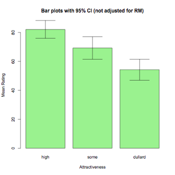
means <- tapply(newData$rate,newData$looks,mean)
sds <- tapply(newData$rate,newData$looks,sd)
barplot2(means,beside=TRUE,main="Bar plots with 95% CI (not adjusted for RM)",
col="lightgreen",ylab="Mean Rating",xlab="Attractiveness",
ci.l=means+((sds/sqrt(num))*qt(0.025,df=(num-1))),
ci.u=means+((sds/sqrt(num))*qt(0.975,df=(num-1))),plot.ci=TRUE)
means <- tapply(newData$rate,newData$charisma,mean)
sds <- tapply(newData$rate,newData$charisma,sd)
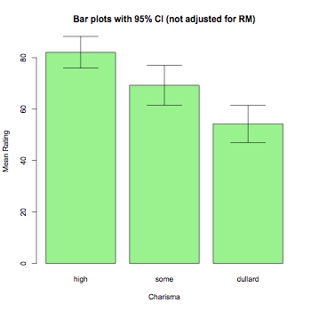
barplot2(means,beside=TRUE,main="Bar plots with 95% CI (not adjusted for RM)",
col="lightgreen",ylab="Mean Rating",xlab="Charisma",
ci.l=means+((sds/sqrt(num))*qt(0.025,df=(num-1))),
ci.u=means+((sds/sqrt(num))*qt(0.975,df=(num-1))),plot.ci=TRUE)
# interaction plots
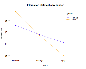
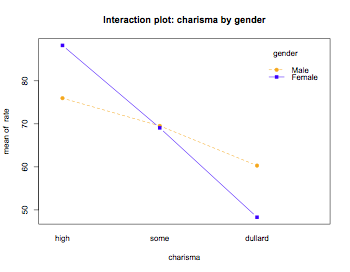
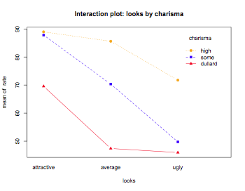
attach(newData)
interaction.plot(looks,gender,rate,main="Interaction plot: looks by gender",type="b",pch=c(19,15),col=c("orange","blue"))
interaction.plot(charisma,gender,rate,main="Interaction plot: charisma by gender",type="b",pch=c(19,15),col=c("orange","blue"))
interaction.plot(looks,charisma,rate,main="Interaction plot: looks by charisma",type="b",pch=c(19,15,17),col=c("orange","blue","red"))
detach(newData)
Mixed-design ANOVA (built-in functions; also, see ez package below)
# read data from local disk
thisData =  read.table("spanengRT.txt", header=TRUE)
thisData$listener = as.factor(thisData$listener)

library(psych)
describe(thisData)

# getting subset of the data
subsetData = subset(thisData,pair=="d_r"|pair=="d_th"|pair=="r_th")
library(gdata)
subsetData = drop.levels(subsetData)

# Mixed-design ANOVA with aov()
# there is no built-in Sphericity test and post-hoc test (TurkeyHSD)
fit = aov(MedianRT ~ (pair*group) + Error(listener/pair), data=subsetData)
summary(fit)

# do Mixed-design ANOVA with lme() in the nlme package
# there is no built-in Sphericity test and post-hoc test (TurkeyHSD)
require(nlme)
fit2 = lme(MedianRT ~ (pair*group), random = ~1|listener/pair, data=subsetData)
summary(fit2)
anova(fit2)

# Need to find out how to do a Mixed-design ANOVA with
# lm()/mlm() (multivariate approach)
Mixed-design ANOVA (using ez package)
# ez() is probably the easiest way to implement mixed-design ANOVA with R
# read data from local disk
thisData =  read.table("spanengRT.txt", header=TRUE)
thisData$listener = as.factor(thisData$listener)
# getting subset of the data
subsetData = subset(thisData,pair=="d_r"|pair=="d_th"|pair=="r_th")
library(gdata)
subsetData = drop.levels(subsetData)

library(ez)
model.ezAnova <- ezANOVA(data=thisData, dv=.(MedianRT), wid=.(listener), within=.(pair), between=.(group))
MinF
# set sum-to-zero
options(contrasts=c("contr.sum","contr.poly"))
thisData = read.csv("langFixFallacyData.csv")
lowIndex = grep("Low[1-9]",colnames(thisData))
highIndex = grep("High[1-9]",colnames(thisData))
subjData = as.data.frame(c(1:10))
subjData$lowFreq = apply(thisData[,lowIndex],1,function(x){mean(x,na.rm=TRUE)})
subjData$highFreq = apply(thisData[,highIndex],1,function(x){mean(x,na.rm=TRUE)})
colnames(subjData) = c("Subj","lowFreq","highFreq")
summary(subjData)
head(subjData)
library(reshape)
subjData = melt(subjData,id="Subj")
subjData$Subj = as.factor(subjData$Subj)
colnames(subjData) = c("Subj","Freq","RT")
head(subjData)
model1 = aov(RT ~ Freq + Error(Subj/Freq), data=subjData)
summary(model1)
pdf("languageFixEffect.pdf", width = 8, height = 6, onefile = TRUE, pointsize = 8)
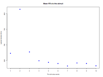
itemMeanScore = apply(thisData[,2:11],2,function(x){mean(x,na.rm=TRUE)})
plot(itemMeanScore, pch=19, col="blue", cex=1.2, lab=c(10,5,7),
main="Mean RTs to the stimuli",ylab="Lexical decision time",
xlab="The stimulus words")
dev.off()
itemData = t(thisData)
itemData = as.data.frame(itemData[-c(1),])
head(itemData)
itemData$Mean = apply(itemData,1,function(x){mean(x,na.rm=TRUE)})
itemData$Freq = gsub("Low[1-9]","low",rownames(itemData))
itemData$Freq = gsub("High[1-9]","high",itemData$Freq)
itemData = subset(itemData,select=c("Mean","Freq"))
head(itemData)
model2 = aov(Mean ~ factor(Freq), data=itemData)
summary(model2)
# Computing MinF (see Brysbaert (2007))
minF = function(F1,F1_df1,F1_df2,F2,F2_df1,F2_df2) {
minF = (F1*F2)/(F1+F2)
minF_df1 = F1_df1
minF_df2 = ((F1+F2)^2)/((F1^2/F2_df2) + (F2^2/F1_df2))
cat("MinF\n\n")
return(list(minF=minF,df1=minF_df1,df2=minF_df2, p=df(minF,minF_df1,minF_df2)))
}
minF(35.646,1,9,2.920,1,8)
Logistic Regression (W14)
logistic regression is implemented with glm() (generalized linear model)
#  Family           Type of regression  Default Link Function
#  ------------------------------------------------------------------
#  binomial         logistic regression binomial("logit")
#  gaussian         Gaussian            gaussian("identity")
#  Gamma            Gamma-distribution  Gamma("inverse")
#  inverse.gaussian inverse Gausian     inverse.gaussian("1/mu^2")
#  poission         -                   poisson("link")
#  quasibinomial    -                   quasibinomial("logit")
#  quasipoisson     -                   quasipoission("log")
logistic regression
library(psych)

thisData = read.csv("DDRASSTR.txt", sep="\t")

thisData$strnumbers = factor(thisData$strnumbers)
thisData$style = factor(thisData$style)
thisData$region = factor(thisData$region)
thisData$banknumbers = factor(thisData$banknumbers)
thisData$classnumbers = factor(thisData$classnumbers)
thisData$participant.number = factor(thisData$participant.number)

summary(thisData)
describe(thisData)

attach(thisData)

table(str,emphatic)

# re-ordering levels
thisData$emphatic = relevel(emphatic,ref="more")

fit1 = glm(str ~ emphatic, data=thisData, family=binomial("logit"))
fit1
# the exponent of coefficients are equal to odds
exp(coef(fit1))

# something is wrong with this. The coefficients do not match with those on the handout
table(str,age,gender)
fit2 = glm(str ~ age*gender-1, data=thisData, family=binomial("logit"))
fit2
| - | to vector | to matrix | to data frame |
| to vector | c(x,y) | cbind(x,y); rbind(x,y) | data.frame(x,y) |
| to matrix | as.vector(myMatrix) | – | as.data.frame(myMatrix) |
| to data frame | – | as.matrix(myDataframe) | – |
Non-parametric tests (W13)
Rank-sum test (Wilcox (rank-sum) test or Mann-Whitney test)
x <- c(1.83,  0.50,  1.62,  2.48, 1.68, 1.88, 1.55, 3.06, 1.30)
y <- c(0.878, 0.647, 0.598, 2.05, 1.06, 1.29, 1.06, 3.14, 1.29)
wilcox.test(x, y, paired = TRUE, alternative = "greater")
Binomial test
# binomial test
binom.test(x=52,n=156,p=.25)
Chisqure test
- Assumptions of chi-square test
- All variables must be categorical
- Random sample data
- Sufficiently large sample in each cell (at least 5 in each cell)
- Independence of each observation
# chi-square test
x = matrix(c(16,4,8,12),nrow=2,byrow=TRUE)
chisq.test(x,correct=FALSE)
Fisher's exact test
TeaTasting <- matrix(c(3, 1, 1, 3), nrow = 2,
	dimnames = list(Guess = c("Milk", "Tea"), Truth = c("Milk", "Tea")))
fisher.test(TeaTasting, alternative = "greater")
Kruskal-Wallis rank sum test
uncooperativeness <- c(6,7,10,8,8,9,8,10,6,8,7,3,7,1)
treatment <- factor(rep(1:3,c(6,4,4)), labels = c("Method A","Method B","Method C"))
uncooperativenessData <- data.frame(uncooperativeness,treatment)

kruskal.test(uncooperativenessData,treatment)

pairwise.t.test(uncooperativeness,treatment,p.adj="bonferroni")
pairwise.t.test(uncooperativeness,treatment,p.adj="holm")
Three-way ANOVA
# loading data (from SPSS)
myData <- read.spss("3wayANOVA.sav",to.data.frame=TRUE)
summary(myData)

# running 3-way ANOVA
attach(myData)
lm.3way <- lm(Depression~Gender*Therapy*Medication)
anova(lm.3way)

# printing an interaction plot
pdf("3wayInteraction.pdf", width = 6, height = 8, onefile = TRUE, pointsize = 9)
par(mfrow=c(2,1))
interaction.plot(Gender,Medication,Depression,col=4:3,fixed=TRUE)
interaction.plot(Gender,Therapy,Depression,col=4:3,fixed=TRUE)
par(mfrow=c(1,1))
dev.off()

detach(myData)
Multilevel Liniear (mixed-effects) Model
Field textbook Ch.19 Multilevel Linear Model (demo using R)
library(foreign); library(lme4);
# see p.733 (but, the data (viagraCovariate.sav) seem to be different on the textbook)
# or something is wrong with the calculation of the fixed intercepts/slopes
thisData <- read.spss("DiscoveryingStatsSPSS3/ViagraCovariate.sav", to.data.frame=TRUE)
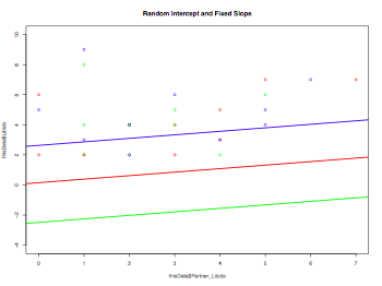
pdf("mixedEffectPlot.pdf", width = 8, height = 6, onefile = TRUE, pointsize = 8)
plot(thisData$Partner_Libido, thisData$Libido, col=rainbow(3), ylim=c(-4,10), main="Random Intercept and Fixed Slope")
model1 <- lm(thisData$Partner_Libido ~ thisData$Libido)
for (i in 1:length(levels(thisData$Dose))) {
thisData.temp <- subset(thisData,Dose==levels(thisData$Dose)[i])
model2 <- lm(thisData.temp$Partner_Libido ~ thisData.temp$Libido)
abline(model2$coefficients[1], model1$coefficients[2], col=rainbow(3)[i], lwd=2)
}
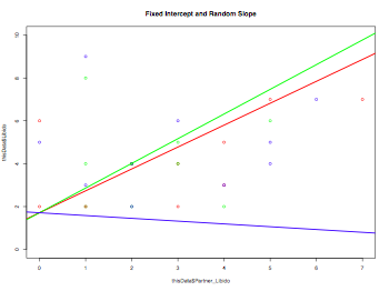
plot(thisData$Partner_Libido, thisData$Libido, col=rainbow(3), ylim=c(0,10), main="Fixed Intercept and Random Slope")
model1 <- lm(thisData$Partner_Libido ~ thisData$Libido)
for (i in 1:length(levels(thisData$Dose))) {
thisData.temp <- subset(thisData,Dose==levels(thisData$Dose)[i])
model2 <- lm(thisData.temp$Partner_Libido ~ thisData.temp$Libido)
abline(model1$coefficients[1], model2$coefficients[2], col=rainbow(3)[i], lwd=2)
}
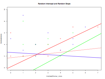
plot(thisData$Partner_Libido, thisData$Libido, col=rainbow(3), ylim=c(0,10), main="Random Intercept and Random Slope")
abline(lm(thisData$Partner_Libido ~ thisData$Libido), col="red")
for (i in 1:length(levels(thisData$Dose))) {
abline(lm(thisData[thisData$Dose==levels(thisData$Dose)[i],"Partner_Libido"] ~
thisData[thisData$Dose==levels(thisData$Dose)[i],"Libido"]), col=rainbow(3)[i], lwd=2)
}
dev.off()
thisData <- read.spss("DiscoveryingStatsSPSS3/Cosmetic Surgery.sav", to.data.frame=TRUE)
# running a simple one-way ANOVA (p.743)
fit1 <- aov(thisData$Post_QoL ~ thisData$Surgery)
summary(fit1)
# simple lm() model without any random effects (the same results as the one-way ANOVA)
# the results are slightly different -- Type II and Type III sums of squres??)
fit2 = lm(Post_QoL~Surgery, data=thisData)
summary(fit2)
# page. 747 (how can I do ANCOVA with R??)
fit3 = lm(Post_QoL~Surgery+Base_QoL+Surgery:Base_QoL, data=thisData)
anova(fit3)
# using lmer() in the nlme package (Clinic is a random effects (intercepts); see p.751)
fit4 = lmer(Post_QoL~(1|Clinic)+Surgery+Base_QoL, data=thisData, REML=FALSE)
print(fit4)
# using lmer() in the nlme package (Clinic is a random effects (intercept & slope); see p.755)
fit5 = lmer(Post_QoL~(Surgery|Clinic)+Surgery+Base_QoL, data=thisData, REML=FALSE)
print(fit5, corr=FALSE)
# using lmer() in the nlme package (Clinic is a random effects; see p.758-760)
fit6 = lmer(Post_QoL~(Surgery|Clinic)+Surgery+Base_QoL+Reason+Surgery:Reason, data=thisData, REML=FALSE)
print(fit6, corr=FALSE)
Data management
Data type conversion
# Converting between the contingency table and the data frame
data = factor(rep(c("A","B","C"), 10), levels=c("A","B","C","D","E"))
data
table(data)
as.data.frame(table(data))
Changing the order of levels
# by default, the order is in the alphabetic order
data = factor(rep(c("A","B","C"), 10))
data
data = factor(rep(c("A","B","C"), 10), levels=c("A","C","B"))
data

# re-ordering levels of one of the factors in the data frame
# don't affect the data themselves -- just only the order of levels
data = as.data.frame(cbind(rep(c("A","B","C"),7),rep(c(1,2,3),7)))
data
summary(data)
data$V1 = factor(data$V1,levels=c("B","C","A"))
data
summary(data)
Convert numeric values to factors
# generating dummy data using rep() and rnorm()
x = c(rep(1:4,each=3),rep(1:4,3),rnorm(12,mean=100,sd=10))
dim(x) = c(12,3) # dim():     # of rows, # of columns
# name the columns
colnames(x) = c("factor1","factor2","interval1")
x = as.data.frame(x)         # changing to a dataframe

x$factor1 = factor(x$factor1,labels=c("high","medHigh","medLow","low"))
x$factor1 = factor(x$factor2,labels=c("prime3","prime2","prime1","unrelated"))

summary(x)
Useful functions (merge)
authors <- data.frame(surname = I(c("Tukey", "Venables", "Tierney", "Ripley", "McNeil")),
	nationality = c("US", "Australia", "US", "UK", "Australia"),
	deceased = c("yes", rep("no", 4)))
books <- data.frame(name = I(c("Tukey", "Venables", "Tierney","Ripley", "Ripley",
	"McNeil", "R Core")),title = c("Exploratory Data Analysis","Modern Applied Statistics ...",
	"LISP-STAT","Spatial Statistics", "Stochastic Simulation","Interactive Data Analysis",
	"An Introduction to R"),other.author = c(NA, "Ripley", NA, NA, NA, NA,
	"Venables & Smith"))

merge(authors, books, by.x = "surname", by.y = "name")
Useful functions (aggregate)
testDF = data.frame(v1 = c(1,3,5,7,8,3,5,NA,4,5,7,9), v2 = c(11,33,55,77,88,33,55,NA,44,55,77,99) )
by1 = c("red","blue",1,2,NA,"big",1,2,"red",1,NA,12)
by2 = c("wet","dry",99,95,NA,"damp",95,99,"red",99,NA,NA)
aggregate(x = testDF, by = list(by1, by2), FUN = "mean")
Useful function (melt)
# transform a data frame to another data frame to compute
# repeated-measure analyses
# make a dummy data set
thisData = rbind(c(4,6,2),c(10,9,8),c(5,4,3),c(8,6,7),c(2,2,2))
thisData = as.data.frame(thisData)
colnames(thisData) = c("early","mid","late")
thisData

library(reshape)
# make a new col to keep the subject id
temp = cbind(thisData,as.factor(rownames(thisData)))
colnames(temp) = c(colnames(thisData),"subject")
melt(temp,id=c("subject"))
Useful function (trimming whitespace)
# trimming whitespace
library(gdata)
myData <- trim(myData)
Graphics
Field textbook Ch.4 Graphics (demo using R)
library(foreign)
thisData <- read.spss("DiscoveryingStatsSPSS3/DownloadFestival.sav", to.data.frame=TRUE)
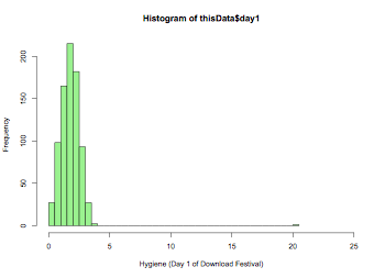
# p.98
hist(thisData$day1,xlim=c(0,25),breaks=50,col="lightgreen",xlab="Hygiene (Day 1 of Download Festival)")
# p.101
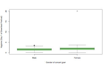
boxplot(thisData$day1~thisData$gender,col="lightgreen",xlab="Gender of concert goer",ylab="Hygiene (Day 1 of Download Festival)")
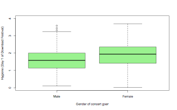
boxplot(thisData$day1~thisData$gender,col="lightgreen",ylim=c(0,4),xlab="Gender of concert goer",ylab="Hygiene (Day 1 of Download Festival)")
# p.106
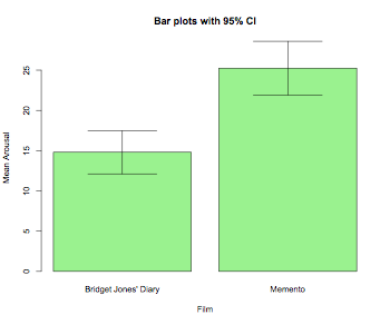
thisData <- read.spss("DiscoveryingStatsSPSS3/ChickFlick.sav", to.data.frame=TRUE)
library(gplots)
num <- tapply(thisData$arousal,thisData$film,length)
means <- tapply(thisData$arousal,thisData$film,mean)
sds <- tapply(thisData$arousal,thisData$film,sd)
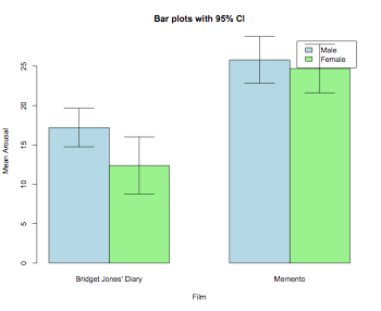
barplot2(means,beside=TRUE,main="Bar plots with 95% CI", col="lightgreen",ylab="Mean Arousal",xlab="Film",
ci.l=means+((sds/sqrt(num))*qt(0.025,df=(num-1))), ci.u=means+((sds/sqrt(num))*qt(0.975,df=(num-1))),plot.ci=TRUE)
# p.108
num <- tapply(thisData$arousal,list(thisData$gender,thisData$film),mean)
means <- tapply(thisData$arousal,list(thisData$gender,thisData$film),mean)
sds <- tapply(thisData$arousal,list(thisData$gender,thisData$film),sd)
barplot2(means,beside=TRUE,main="Bar plots with 95% CI", col=c("lightblue","lightgreen"),ylab="Mean Arousal",
xlab="Film", ci.l=means+((sds/sqrt(num))*qt(0.025,df=(num-1))), ci.u=means+((sds/sqrt(num))*qt(0.975,df=(num-1))),
plot.ci=TRUE,legend=levels(thisData$gender))
# p.118
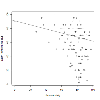
thisData <- read.spss("DiscoveryingStatsSPSS3/Exam Anxiety.sav", to.data.frame=TRUE)
# the regression line differs from one in the textbook. I don't know why.
plot(thisData$Anxiety,thisData$Exam,ylab="Exam Performance (%)",xlab="Exam Anxiety")
abline(lm(thisData$Anxiety~thisData$Exam))
# p.121
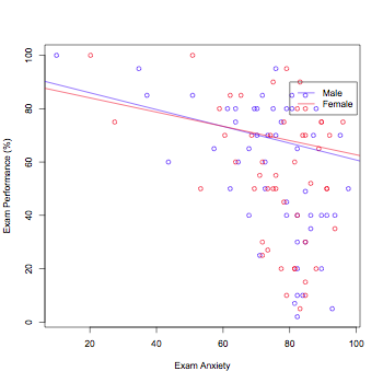
thisData.male <- subset(thisData,Gender=="Male")
thisData.female <- subset(thisData,Gender=="Female")
plot(thisData.male$Anxiety,thisData.male$Exam,col="blue",ylab="Exam Performance (%)",xlab="Exam Anxiety")
points(thisData.female$Anxiety,thisData.female$Exam,col="red")
abline(lm(thisData.male$Anxiety~thisData.male$Exam),col="blue")
abline(lm(thisData.female$Anxiety~thisData.female$Exam),col="red")
legend(80,90,c("Male","Female"),col=c("blue","red"),lty=1)
# p.123
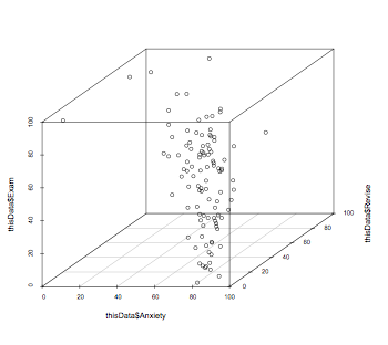
library(scatterplot3d)
scatterplot3d(thisData$Anxiety,thisData$Revise,thisData$Exam)
# p.125
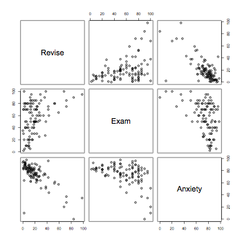
pairs(thisData[,c("Revise","Exam","Anxiety")])
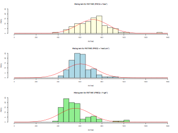
Histogram
myData = read.delim("Rxtime.dat",header = TRUE, sep = "\t", quote="\"", dec=".")

# fixing the labels of nominal variabls
myData$FREQ = factor(myData$FREQ,labels=c("high","medium","low"))
myData$PRIME_YESNO = factor(myData$PRIME_YESNO,labels=c("prime","unrelated"))

summary(myData)

pdf("histogram.pdf", width = 8, height = 6, onefile = TRUE, pointsize = 8)
par(mfrow=c(3,1))
hist(myData[myData$FREQ=="low",]$RXTIME,xlim=c(0,1400),ylim=c(0,25),
                breaks=c(50*0:28),main="Histogram for RXTIME (FREQ = 'low'')",
                xlab="RXTIME",ylab="FREQ",col="lightyellow")
# see the R Book p.214
# the density function must be multiplied by the total freq by the width
# of the bin
xv = seq(0,1400,10)
yv = dnorm(xv,mean(myData[myData$FREQ=="low",]$RXTIME), sd(myData[myData$FREQ=="low",]$RXTIME))*100*50
lines(xv,yv,col="red")
hist(myData[myData$FREQ=="medium",]$RXTIME,xlim=c(0,1400),ylim=c(0,25),
                breaks=c(50*0:28),main="Histogram for RXTIME (FREQ = 'med'')",
                xlab="RXTIME",ylab="FREQ",col="lightblue")

xv = seq(0,1400,10)
yv = dnorm(xv,mean(myData[myData$FREQ=="medium",]$RXTIME), sd(myData[myData$FREQ=="low",]$RXTIME))*100*50
lines(xv,yv,col="red")
hist(myData[myData$FREQ=="high",]$RXTIME,xlim=c(0,1400),ylim=c(0,25),
                breaks=c(50*0:28),main="Histogram for RXTIME (FREQ = 'high'')",
                xlab="RXTIME",ylab="FREQ",col="lightgreen")

xv = seq(0,1400,10)
yv = dnorm(xv,mean(myData[myData$FREQ=="high",]$RXTIME), sd(myData[myData$FREQ=="low",]$RXTIME))*100*50
lines(xv,yv,col="red")
par(mfrow=c(1,1))
dev.off()
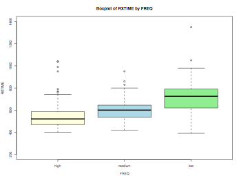
Boxplot
myData = read.delim("Rxtime.dat",header = TRUE, sep = "\t", quote="\"", dec=".")

# fixing the labels of nominal variabls
myData$FREQ = factor(myData$FREQ,labels=c("high","medium","low"))
myData$PRIME_YESNO = factor(myData$PRIME_YESNO,labels=c("prime","unrelated"))

summary(myData)

color = c("lightyellow","lightblue","lightgreen")

pdf("corpusAnalysisHW2Boxplot.pdf", width = 8, height = 6, onefile = TRUE, pointsize = 8)
boxplot(myData$RXTIME~myData$FREQ,main="Boxplot of RXTIME by FREQ", ylim=c(200,1400),xlab="FREQ",ylab="RXTIME",col=color)
dev.off()
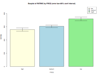
Bar chart (with conf intervals)
myData = read.delim("Rxtime.dat",header = TRUE, sep = "\t", quote="\"", dec=".")

# fixing the labels of nominal variabls
myData$FREQ = factor(myData$FREQ,labels=c("high","medium","low"))
myData$PRIME_YESNO = factor(myData$PRIME_YESNO,labels=c("prime","unrelated"))

summary(myData)

color = c("lightyellow","lightblue","lightgreen")

# error bar 95% confidence interval using gplots function 'barplot2'
library(gplots)
pdf("barchart.pdf", width = 8, height = 6, onefile = TRUE, pointsize = 8)
tempData = tapply(myData$RXTIME,myData$FREQ,mean)
tempData2 = tapply(myData$RXTIME,myData$FREQ,sd)
n = tapply(myData$RXTIME,myData$FREQ,length)

barplot2(tempData,ylim=c(0,900),beside=TRUE,
                main="Boxplot of RXTIME by FREQ (error bar=95% conf interval)",
                ylab="RXTIME",xlab="FREQ",col=color,
                ci.l=tempData+((tempData2/sqrt(n))*qt(0.025,df=(n-1))),
                ci.u=tempData+((tempData2/sqrt(n))*qt(0.975,df=(n-1))),
                plot.ci=TRUE)

labs = c("low","medium","hight")
legend("topright",labs,fill=color)
dev.off()
Bar chart (with conf intervals adjusted for RM)
# makeing an adjusted bar plot (Field's book pp.317-324)

library(foreign)
library(gplots)
thisData <- read.spss( "DiscoveryingStatsSPSS3/spiderRM.sav", to.data.frame=TRUE)
thisData <- thisData[c(1:12),]
thisData$subject <- as.factor(rownames(thisData))

num <- length(thisData$subject)
means <- mean(thisData[,c("picture","real")])
sds <- sd(thisData[,c("picture","real")])
# this is not adjusted for RM measures
barplot2(means,beside=TRUE,main="Bar plots with 95% CI",col="lightyellow",ylab="Mean",
	xlab="Treatment",ci.l=means+((sds/sqrt(num))*qt(0.025,df=(num-1))),
	ci.u=means+((sds/sqrt(num))*qt(0.975,df=(num-1))),plot.ci=TRUE)

# calculating adjustment
# (1) calculating the mean for each participant
indM <- apply(thisData[,c("picture","real")],1,mean)
# (2) calculate the grand mean
grandM <- mean(apply(thisData[,c("picture","real")],1,mean))
# (3)/(4) calculate adjustment (grand mean - individual mean)
adjustment <- grandM - indM

# this is ajusted for RM
num <- length(thisData$subject)
means <- mean(thisData[,c("picture","real")] + adjustment)
sds <- sd(thisData[,c("picture","real")] + adjustment)
barplot2(means,beside=TRUE,main="Bar plots with 95% CI (adjusted for RM)",
	col="lightyellow",ylab="Mean",xlab="Treatment",
	ci.l=means+((sds/sqrt(num))*qt(0.025,df=(num-1))),
	ci.u=means+((sds/sqrt(num))*qt(0.975,df=(num-1))),plot.ci=TRUE)
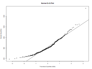
QQplot
myData = read.delim("Rxtime.dat",header = TRUE, sep = "\t", quote="\"", dec=".")

# fixing the labels of nominal variabls
myData$FREQ = factor(myData$FREQ,labels=c("high","medium","low"))
myData$PRIME_YESNO = factor(myData$PRIME_YESNO,labels=c("prime","unrelated"))

summary(myData)

pdf("qqplot.pdf", width = 8, height = 6, onefile = TRUE, pointsize = 8)
qqplot(rt(1000,df=99), myData$RXTIME, main = "Normal Q-Q Plot",
            xlab = "Theoretical Quantiles (t(99))",
            ylab = "Sample Quantiles", plot.it = TRUE)
qqline(myData$RXTIME)
dev.off()
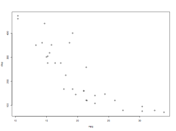
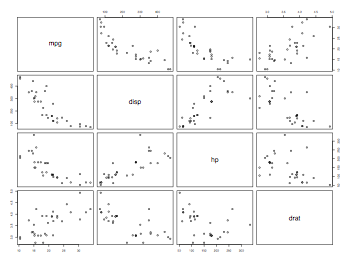
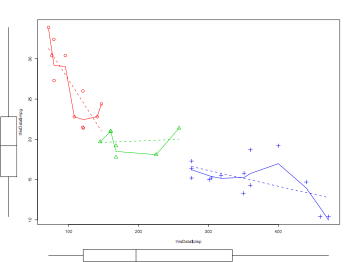
Scatterplot
# not from the textbook
thisData = read.table("mtcars.txt",header=TRUE)
attach(thisData)

pdf("scatterplotsPlot.pdf", width = 8, height = 6, onefile = TRUE, pointsize = 8)
plot(thisData[,c("mpg","disp")])
dev.off()

pdf("scatterplotsPairs.pdf", width = 8, height = 6, onefile = TRUE, pointsize = 8)
pairs(thisData[,c("mpg","disp","hp","drat")])
dev.off()

pdf("scatterplotsCarPackage.pdf", width = 8, height = 6, onefile = TRUE, pointsize = 8)
# with the car package
scatterplot(thisData$disp, thisData$mpg, group=thisData$cyl,cex=1.5)
dev.off()

pdf("scatterplotsMatrix.pdf", width = 8, height = 6, onefile = TRUE, pointsize = 8)
# with the car package
scatterplot.matrix(~mpg+disp+hp|cyl, data=thisData)
dev.off()
detach()
Putting the axis labels on the plot in different angles (45 or vertical)
thisData = read.table("mtcars.txt",header=TRUE)
attach(thisData)
pdf("scatterplotsPlotWithAngledAxisLabel.pdf", width = 8, height = 6, onefile = TRUE, pointsize = 8)
plot(thisData[,c("mpg","disp")], xaxt="n", xlim=c(10,35))
labelList = as.vector(c(10:35))
text(x=seq(10,35,by=1), par("usr")[3] - 10, labels = labelList, srt = 45, pos = 1, xpd = TRUE)
dev.off()
detach()
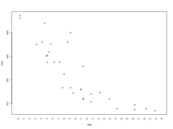
Distributions
Shading the critical areas in the distribution
# Density for nomal distribution
# shade.tails() from Quantitative Methods in Linguistics Ch.1
#------- shade.tails -------------------
# draw probability density functions of t with critical regions shaded.
#   by default the function draws the 95% confidence interval on the normal
#   distribution.
#
# Input parameters
#    crit - the critical value of t (always a positive number)
#    df - degrees of freedom of the t distribution
#    tail - "upper", "lower" or "both"
#    xlim - the x axis range is -xlim to +xlim

shade.tails = function(crit=1.96, df = 10000, tail = "both",xlim=3.5) {
    curve(dt(x,df),-xlim,xlim,ylab="Density",xlab="t")
    ylow = dt(xlim,df)
    pcrit = pt(crit,df)
    caption = paste(signif(1-pcrit,3))

    if (tail  "both" | tail  "lower") {
        xx = seq(-xlim,-crit,0.05)
        yy = dt(xx,df)
        polygon(c(xx,-crit,-xlim),c(yy,ylow,ylow),density=20,angle = -45)
        text(-crit-0.7,dt(crit,df)+0.02,caption)
    }
    if (tail "both" | tail  "upper") {
        xx2 = seq(crit,xlim,0.05)
        yy2 = dt(xx2,df)
        polygon(c(xx2,xlim,crit),c(yy2,ylow,ylow),density=20,angle = 45)
        text(crit+0.7,dt(crit,df)+0.02,caption)
    }
}
x = sort(rnorm(10000))
hx = dnorm(x,mean(x),sd(x))
pdf("shadeInDistribution.pdf", width = 8, height = 6, onefile = TRUE, pointsize = 8)
plot(x, hx, type="n", xlab="", ylab="Density", main="Normal Distribution (n=10000, crit = 1.96)")
lines(x,hx)
shade.tails()
dev.off()
Correlation and Regression
x = c(1:6)
y = c(.44,.515,.55,.575,.605,.615)
x - mean(x)
y - mean(y)

sumOfDeviationProd = sum((x - mean(x))*(y - mean(y)))
covariance = sumOfDeviationProd/(length(x)-1)
r = covariance/(sd(x)*sd(y))
t = (r-0)/sqrt((1-r^2)/(length(x)-2))

cat("Sum of Deviation Products:",sumOfDeviationProd,"\n",
    "Covariance               :",covariance,"\n",
    "r                        :",r,"\n",
    "t                        :",t,"\n"
    ,sep="")

cor(x,y)
cov(x,y)
cor.test(x,y)
Time Series
Analyzing the New York Times' COVID-19 data with the Time Series (zoo) package
library(zoo)

# Read the New York Times' COVID-19 data. This may take some time depending on the Internet speed
thisData <- read.csv("https://raw.githubusercontent.com/nytimes/covid-19-data/master/us-counties.csv", sep = ",")
thisData$county <- as.factor(thisData$county)
thisData$state <- as.factor(thisData$state)
thisData$date <- as.Date(thisData$date)
summary(thisData)

# Creating a Time Series object only for NYC
temp <- droplevels(thisData[thisData$county=="New York City",])
temp$caseInc <- c(diff(as.numeric(temp$cases)),0)
temp$deathsInc <- c(diff(as.numeric(temp$deaths)),0)
thisTS.caseInc <- read.zoo(temp[,c("date","caseInc")], index.column=1)
summary(thisTS.caseInc)

# calculating the 7 days average
thisTS.caseIncAve <- rollmean(thisTS.caseInc,7,align="center")

# plotting the data
plot.zoo(thisTS.caseIncAve,xlab="Date",xaxt="n", ylab="COVID-19 Cases", main="COVID-19 Cases (weekly average) in New York City\nData: the New York Times (https://github.com/nytimes/covid-19-data)")
thisTS.caseIncAve.Date <- seq(as.Date("2020-3-1"), as.Date("2021-12-1"), by = "month")
text(thisTS.caseIncAve.Date, par("usr")[3] - 300, labels = thisTS.caseIncAve.Date, srt = 45, pos = 1, xpd = TRUE, cex=0.8)